In a study recently published in JGR Oceans, we extended ambient noise interferometry to ocean surface gravity waves (OSGW) observed on a DAS array in shallow water. Extracting the OSGW Green's function every half hour between each pair of channels, we applied a subarray beamforming method to measure OSGW dispersion and invert for water depth, which may be helpful in locating subsea cables and co-registering optical/geographic channel locations when the cable path is unknown or unavailable. We then applied a waveform stretching method to estimate the Doppler shift between waves propagating in each direction along the array, recovering the depth-averaged along-cable ocean current velocity, which compared favorably to a tidal flow model.
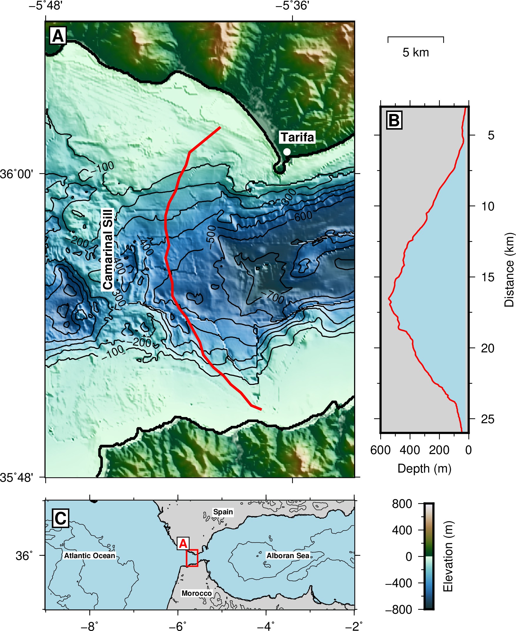
DAS array location along a power cable in the Strait of Gibraltar, offshore southern Spain. We only use the 3-6 km cable segment on the Spanish shelf, where a broad band of OSGW can be observed at the seafloor.
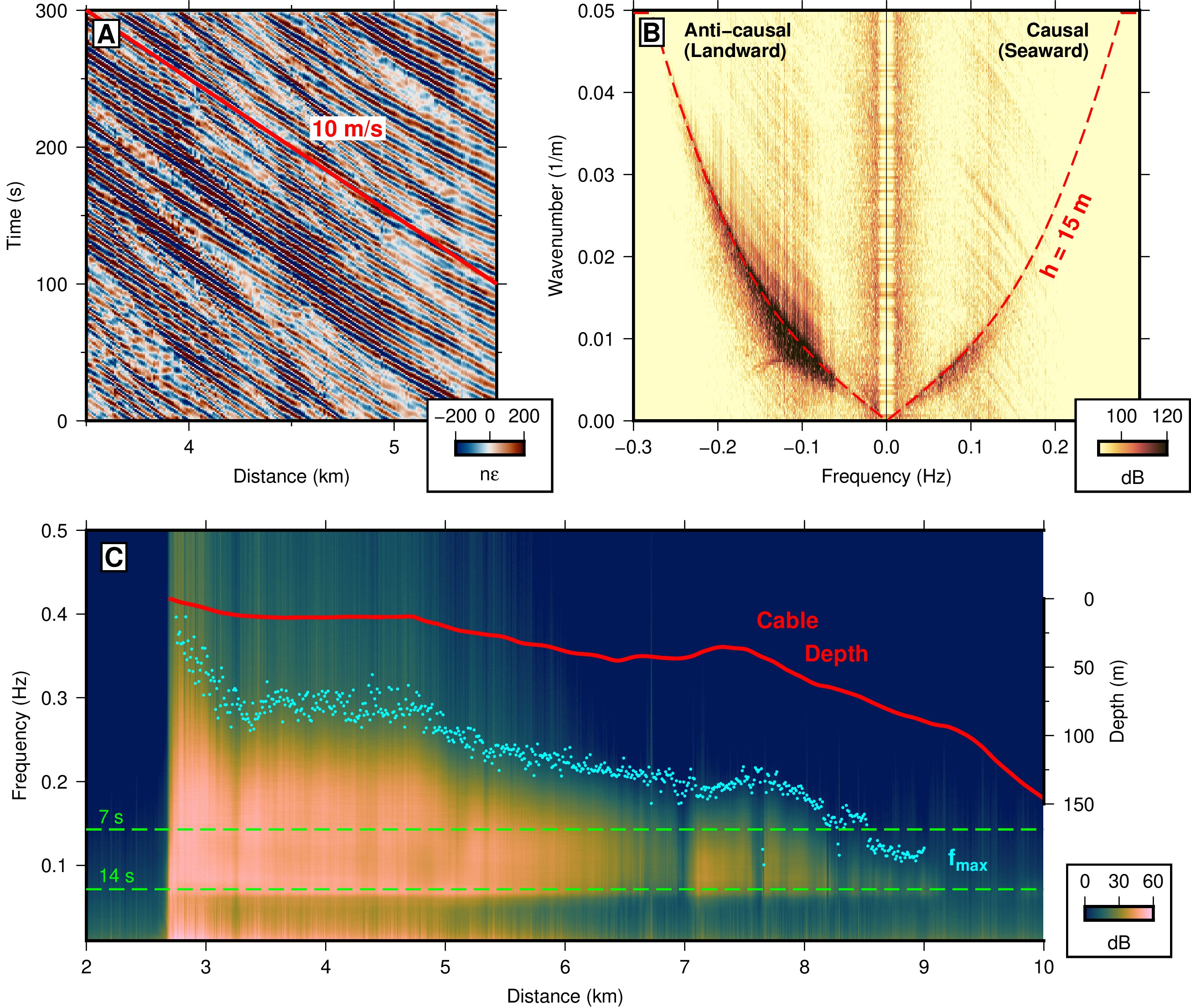
OSGWs in DAS data. (A) Raw time-domain data showing groups of OSGW propagating towards shore at a phase speed around 10 m/s. If you squint, you can see that some waves are also propagating in the opposite direction, but are much weaker. (B) Frequency-wavenumber spectrum of the data showing the classic OSGW dispersion relation. (C) Variation in power spectral density with depth, showing that the maximum frequency and the amplitude are both modulated by water depth, with OSGW signals disappearing between 150-200 m.
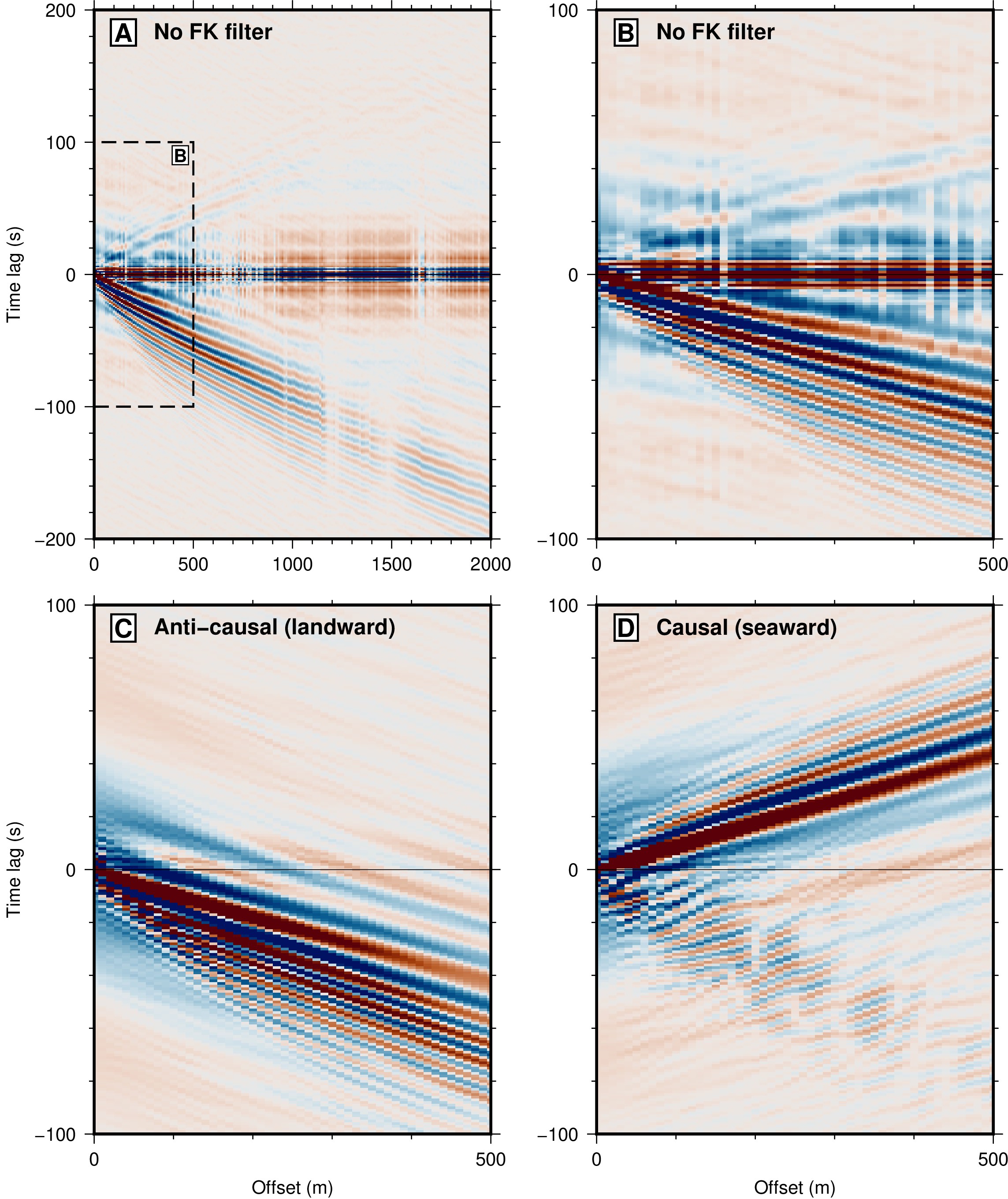
A virtual source gather (the cross-correlation of one channel with many adjacent channels) showing the OSGW Green's function recovered with ambient noise interferometry. In order to measure a Doppler shift, we needed to balance the strong energy propagating towards shore with the weak energy propagating away, so we applied a frequency-wavenumber filter and split the processing into two parallel workflows.
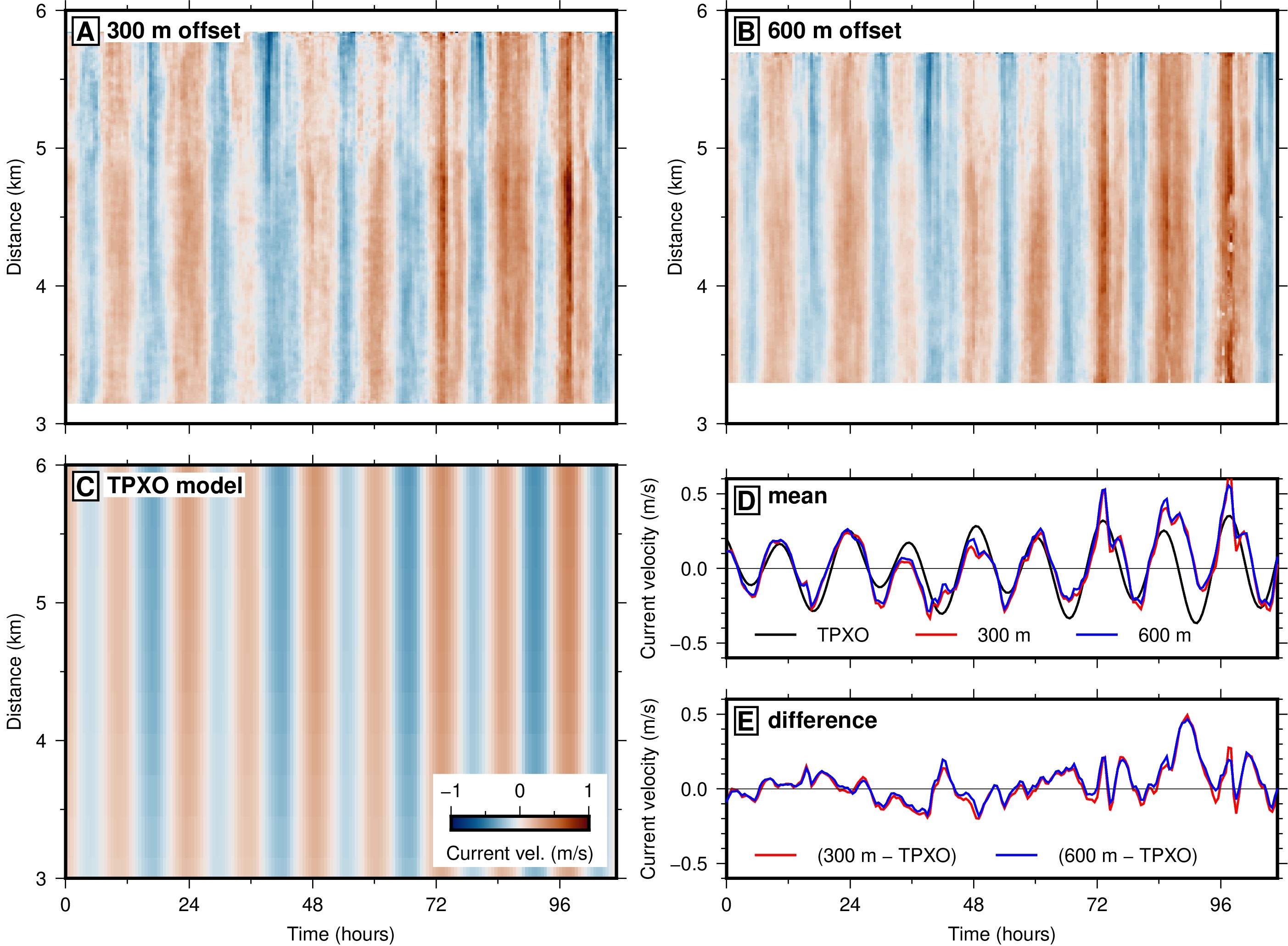
The results of the waveform stretching method, showing the along-cable current velocity as a function of time and space. In (A) and (B), we simply calculated the difference between channel pairs of constant offset. While it is possible to further refine this with tomography, the problem is highly overdetermined and would require strong regularization for very little improvement (given how spatially smooth the results already are). In (C), (D), and (E) we compare the results with the shallow-water predictions for barotropic tidal flow based on the TPXO9 harmonic constituents, showing a great correlation.